Growth Models

The models module contains functions for fitting and selecting growth models to growth curve data.

This module contains:

• fit_model() is the main function of the model; it fits growth models to growth curve data.

• Growth functions (*_function) are Python function in which the first argumet is time and the rest of the argument are model parameters. Time can be given an a numpy.ndarray.

• Growth models (*_model) are lmfit.model.Model objects from the lmfit package. These objects wrap the growth functions and are used to fit models to data with parameter constraints and some useful statistics and models selection methods.

• Parameter guessing functions (guess_*) are function that use the shape of a growth curve to guess growth parameters without fitting a model to the data, but rather through analytic properties of the growth functions.

• Hypothesis testing (has_*) are functions that perform a statistical test to decide if a property of one model can be significantly observed in the data.

• Outlier functions (find_outliers*) are functions for identification of outlier growth curve in high-throughput data sets.

• Indirect trait calculation (find_*) are functions for calculating growth parameters that are indirectly represented by the models.

• and some other utilities.

Models

Curveball uses the logistic model and its derivaties, the Richards model and the Baranyi-Roberts model:

Logistic model

Also known as the Valhulst model, the logistic model includes three parameters and is the simplest and most commonly used population growth model.

The logistic model is defined by an ordinary differential equation (ODE) which also has a closed form solution:

\[ \begin{align}\begin{aligned} \frac{dN}{dt} = r N \Big(1 - \frac{N}{K}\Big) \Rightarrow\\N(t) = \frac{K}{1 - \Big(1 - \frac{K}{N_0} \Big)e^{-r t}}\end{aligned}\end{align} \]

• N: population size

• \(N_0\): initial population size

• r: initial per capita growth rate

• K: maximum population size

Richards model

Also known as the Generalised logistic model, Richards model [Richards1959] (or in its discrete time version, the \(\theta\)-logistic model [Gilpin1973]) extends the logistic model by including the curvature parameter \(\nu\):

\[ \begin{align}\begin{aligned}\frac{dN}{dt} = r N \Big( 1 - \Big(\frac{N}{K}\Big)^{\nu} \Big) \Rightarrow\\N(t) = \frac{K}{\Big[1 - \Big(1 - \Big(\frac{K}{N_0}\Big)^{\nu}\Big) e^{-r \nu t}\Big]^{1/\nu}}\end{aligned}\end{align} \]

• \(y_0\): initial population size

• r: initial per capita growth rate

• K: maximum population size

• \(\nu\): curvature of the logsitic term

The logistic model is then a special case of the Richards model for \(\nu=1\), that is, the Logistic model is nested in the Richards model.

When \(\nu>1\), the effect of the logistic term \((1-(\frac{N}{K})^{\nu})\) increases in comparison to the logistic model, and the transition from fast growth to slow growth is faster.

When \(0<\nu<1\), the effect of the logistic term \((1-(\frac{N}{K})^{\nu})\) decreases in comparison to the logistic model, and the transition from fast growth to slow growth is faster.

Baranyi-Roberts model

The Baranyi-Roberts model [Baranyi1994] extends Richards model by introducing a lag phase in which the population growth is slower than expected while it is adjusting to a new environment. This extension is done by introducing and adjustment function, \(\alpha(t)\):

\[\alpha(t) = \frac{q_0}{q_0 + e^{-v t}}\]

where \(q_0\) is the initial ajdustment of the population and \(v\) is the adjustment rate.

The model is then described by the following ODE and exact solution:

\[ \begin{align}\begin{aligned} \frac{dN}{dt} = r \alpha(t) N \Big( 1 - \Big(\frac{N}{K}\Big)^{\nu} \Big) \Rightarrow\\ N(t) = \frac{K}{\Big[1 - \Big(1 - \Big(\frac{K}{N_0}\Big)^{\nu}\Big) e^{-r \nu A(t)}\Big]^{1/\nu}}\\A(t) = \int_0^t{\alpha(s)ds} = \int_0^t{\frac{q_0}{q_0 + e^{-v s}} ds} = t + \frac{1}{v} \log{\Big( \frac{e^{-v t} + q_0}{1 + q_0} \Big)}\end{aligned}\end{align} \]

• \(N_0\): initial population size

• r: initial per capita growth rate

• K: maximum population size

• \(\nu\): curvature of the logsitic term

• \(q_0\): initial adjustment to current environment

• v: adjustment rate

Note that \(A(t) - t \to \lambda\) as \(t \to \infty\); this \(\lambda\) is called the lag duration.

Richards model is then a special case of the Baranyi-Roberts model for \(1/v \to 0\), that is, Richards model is nested in Baranyi-Roberts. Therefore, Logistic is also nested in Baranyi-Roberts by \(\nu=1, 1/v \to 0\).

Logistic models with lag phase

We define tow additional models: Baranyi-Roberts with \(\nu=1\) or a logistic model with lag phase, and the same model with \(v=r\) [Baty2004]. These models have five and four and parameters, respectively.

Model hierarchy and the likelihood ratio test

The nesting hierarchy between the models is given in Fig. 1. This nesting is used for the Likelihood ratio test using the function curveball.models.lrtest() in which the nested model (to which the arrows point) is the first argument m0, and the nesting model (from which the arrow points) is the second argument m1.

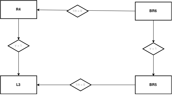
Fig. 6 Fig. 1 - Map of model nesting for the likelihood ratio test.

Parameter guessing

Before fitting models to the data, Curveball attempts to guess the growth parameters from the shape of the curve. These guesses are used as initial parameters in the model fitting procedure.

y0 and K are guessed from the minimum and maximum of the growth curve, respectively.

r and nu are guessed in guess_r() and guess_nu(), respectively, using formulas from [Richards1959]:

\[ \begin{align}\begin{aligned}N_{max} = K (1 + \nu)^{-\frac{1}{\nu}} \Rightarrow\\\frac{dN}{dt}_{max} = r K \nu (1 + \nu)^{-\frac{1 + \nu}{\nu}}\end{aligned}\end{align} \]

• \(\frac{dN}{dt}_{max}\): maximum population growth rate

• \(N_{max}\): population size/density when the population growth rate (\(\frac{dN}{dt}\)) is maximum

• r: initial per capita growth rate

• K: maximum population size

• \(\nu\): curvature of the logsitic term

q0 and v, the lag phase parameters, are guessed by fitting a Baranyi-Roberts model with fixed y0, r, K, and nu (based on guesses) to the data.

Model selection

Model selection is done by comparing the Bayesian Information Criteria (BIC) of all model fits and choosing the model fit with the lowest BIC value. BIC is a common method to measure the quality of a model fit [Kaas1995], balancing between model fit (distance from data) and complexity (number of parameters). See lmfit.model.ModelFit.bic() for more information.

Curveball also calculates the weighted BIC each model fitted to the same data. This can be interpreted as the weight of evidence for each model.

Example

>>> import pandas as pd
>>> import curveball
>>> plate = pd.read_csv('plate_templates/G-RG-R.csv')
>>> df = curveball.ioutils.read_tecan_xlsx('data/Tecan_280715.xlsx', label='OD', plate=plate)
>>> models, fig, ax = curveball.models.fit_model(df[df.Strain == 'G'], PLOT=True, PRINT=False)

Fig. 7 Fig. 2 - Model fitting and selection. The figure is the result of calling fig.savefig() on the result of the above example code. Red error bars: mean and standard deviation of data; Green solid line: model fit; Blue dashed line: initial guess.

References

Richards1959(1,2)

Richards, F. J., 1959. A Flexible Growth Function for Empirical Use. Journal of Experimental Botany

Baranyi1994

Baranyi, J., Roberts, T. A., 1994. A dynamic approach to predicting bacterial growth in food. Int. J. Food Microbiol.

Kaas1995

Kass, R., Raftery, A., 1995. Bayes Factors. J. Am. Stat. Assoc.

Gilpin1973

Gilpin, M. E., Ayala, F. J., 1973. Global Models of Growth and Competition. Proc. Nat. Acad. Sci. U S A.

Baty2004

Baty, Florent, and Marie-Laure Delignette-Muller. 2004. Estimating the Bacterial Lag Time: Which Model, Which Precision?. Intl. J. Food Microbiol.

Members

curveball.models.bootstrap_params(df, model_result, nsamples, unit='Well', fit_kws=None)

Sample model parameters by fitting the model to resampled data.

The data is bootstraped by drawing growth curves (sampling from the unit column in df) with replacement.

dfpandas.DataFrame

the data to fit

model_resultlmfit.model.ModelResult

result of fitting a lmfit.model.Model to data in df

nsamplesint

number of samples to draw

unitstr, optional

the name of the column in df that identifies a resampling unit, defaults to Well

fit_kwsdict, optional

dict of kwargs for fit_model

pandas.DataFrame

data frame of samples; each row is a sample, each column is a parameter.

ValueError : if model_result isn’t an instance of lmfit.model.ModelResult ValueError : if df is empty

sample_params

curveball.models.calc_weights(df, PLOT=False)

Calculate weights for the fittiing procedure based on the standard deviations at each time point.

If there is more than one replicate, use the standard deviations as weight. Warn about NaN and infinite values.

dfpandas.DataFrame

data frame with Time and OD columns

PLOTbool, optional

if True, plot the weights by time

weightsnp.ndarray

array of weights, calculated as the inverse of the standard deviations at each time point

figmatplotlib.figure.Figure

if the argument PLOT was True, the generated figure.

axmatplotlib.axes.Axes

if the argument PLOT was True, the generated axis.

curveball.models.cooks_distance(df, model_fit, use_weights=True)

Calculates Cook’s distance of each well given a specific model fit.

Cook’s distance is an estimate of the influence of a data curve when performing model fitting; it is used to find wells (growth curve replicates) that are suspicious as outliers. The higher the distance, the more suspicious the curve.

dfpandas.DataFrame

growth curve data, see curveball.ioutils for a detailed definition.

model_fitlmfit.model.ModelResult

result of model fitting procedure

use_weightsbool, optional

should the function use standard deviation across replicates as weights for the fitting procedure, defaults to True.

dict

a dictionary of Cook’s distances: keys are wells (from the Well column in df), values are Cook’s distances.

Wikipedia

curveball.models.find_K_ci(param_samples, ci=0.95)

Estimates a confidence interval for K, the maximum population density from the model fit.

The confidence interval of the doubling time is the lower and higher percentiles such that ci percent of the max densities are within the confidence interval.

param_samplespandas.DataFrame

parameter samples, generated using :function:`sample_params` or :function:`bootstrap_params`

cifloat, optional

the fraction of doubling times that should be within the calculated limits. 0 < ci <, defaults to 0.95.

low, highfloat

the lower and the higher boundaries of the confidence interval of the maximum population density.

curveball.models.find_all_outliers(df, model_fit, deviations=2, max_outlier_fraction=0.1, use_weights=True, PLOT=False)

Iteratively find outlier wells in growth curve data.

At each iteration, calls find_outliers(). Iterations stop when no more outliers are found or when the fraction of wells defined as outliers is above max_outlier_fraction.

dfpandas.DataFrame

growth curve data, see curveball.ioutils for a detailed definition.

model_fitlmfit.model.ModelResult

result of model fitting procedure

deviationsfloat, optional

the number of standard deviations that defines an outlier, defaults to 2.

max_outlier_fractionfloat, optional

maximum fraction of wells to define as outliers, defaults to 0.1 = 10%.

use_weightsbool, optional

should the function use standard deviation across replicates as weights for the fitting procedure, defaults to True.

axmatplotlib.axes.Axes

an axes to plot into; if not provided, a new one is created.

PLOTbool, optional

if True, the function will plot the Cook’s distances of the wells and the threshold.

outlierslist

a list of lists: the list nested at index i contains the labels of the outlier wells found at iteration i.

figmatplotlib.figure.Figure

if the argument PLOT was True, the generated figure.

axmatplotlib.axes.Axes

if the argument PLOT was True, the generated axis.

curveball.models.find_lag(model_fit, params=None)

Estimates the lag duration from the model fit.

The function calculates the tangent line to the model curve at the point of maximum derivative (the inflection point). The time when this line intersects with \(N_0\) (the initial population size) is labeled \(\lambda\) and is called the lag duration time [fig2.2].

model_fitlmfit.model.ModelResult

the result of a model fitting procedure

paramslmfit.parameter.Parameters, optional

if provided, these parameters will override model_fit’s parameters

lamfloat

the lag phase duration in the units of the model_fit Time variable (usually hours).

fig2.2

Fig. 2.2 pg. 19 in Baranyi, J., 2010. Modelling and parameter estimation of bacterial growth with distributed lag time..

find_lag_ci has_lag

curveball.models.find_lag_ci(model_fit, param_samples, ci=0.95)

Estimates a confidence interval for the lag duration from the model fit.

The lag duration for each parameter sample is calculated. The confidence interval of the lag is the lower and higher percentiles such that ci percent of the random lag durations are within the confidence interval.

model_fitlmfit.model.ModelResult

the result of a model fitting procedure

param_samplespandas.DataFrame

parameter samples, generated using :function:`sample_params` or :function:`bootstrap_params`

cifloat, optional

the fraction of lag durations that should be within the calculated limits. 0 < ci <, defaults to 0.95.

low, highfloat

the lower and the higher boundaries of the confidence interval of the lag phase duration in the units of the model_fit Time variable (usually hours).

find_lag has_lag

curveball.models.find_max_growth(model_fit, params=None, after_lag=True)

Estimates the maximum population and specific growth rates from the model fit.

The function calculates the maximum population growth rate \(a=\max{\frac{dy}{dt}}\) as the derivative of the model curve and calculates its maximum. It also calculates the maximum of the per capita growth rate \(\mu = \max{\frac{dy}{y \cdot dt}}\). The latter is more useful as a metric to compare different strains or treatments as it does not depend on the population size/density.

For example, in the logistic model the population growth rate is a quadratic function of \(y\) so the maximum is realized when the 2nd derivative is zero:

\[ \begin{align}\begin{aligned}\frac{dy}{dt} = r y (1 - \frac{y}{K}) \Rightarrow\\\frac{d^2 y}{dt^2} = r - 2\frac{r}{K}y \Rightarrow\\\frac{d^2 y}{dt^2} = 0 \Rightarrow y = \frac{K}{2} \Rightarrow\\\max{\frac{dy}{dt}} = \frac{r K}{4}\end{aligned}\end{align} \]

In contrast, the per capita growth rate a linear function of \(y\) and so its maximum is realized when \(y=y_0\):

\[ \begin{align}\begin{aligned}\frac{dy}{y \cdot dt} = r (1 - \frac{y}{K}) \Rightarrow\\\max{\frac{dy}{y \cdot dt}} = \frac{dy}{y \cdot dt}(y=y_0) = r (1 - \frac{y_0}{K}) \end{aligned}\end{align} \]

model_fitlmfit.model.ModelResult

the result of a model fitting procedure

paramslmfit.parameter.Parameters, optional

if provided, these parameters will override model_fit’s parameters

after_lagbool

if true, only explore the time after the lag phase. Otherwise start at time zero. Defaults to True.

t1float

the time when the maximum population growth rate is achieved in the units of the model_fit Time variable.

y1float

the population size or density (OD) for which the maximum population growth rate is achieved.

afloat

the maximum population growth rate.

t2float

the time when the maximum per capita growth rate is achieved in the units of the model_fit Time variable.

y2float

the population size or density (OD) for which the maximum per capita growth rate is achieved.

mufloat

the the maximum specific (per capita) growth rate.

find_max_growth_ci

curveball.models.find_max_growth_ci(model_fit, param_samples, after_lag=True, ci=0.95)

Estimates a confidence interval for the maximum population/specific growth rates from the model fit.

The maximum population/specific growth rate for each parameter sample is calculated. The confidence interval of the rate is the lower and higher percentiles such that ci percent of the random rates are within the confidence interval.

model_fitlmfit.model.ModelResult

the result of a model fitting procedure

param_samplespandas.DataFrame

parameter samples, generated using :function:`sample_params` or :function:`bootstrap_params`

after_lagbool

if true, only explore the time after the lag phase. Otherwise start at time zero. Defaults to True

cifloat, optional

the fraction of lag durations that should be within the calculated limits. 0 < ci <, defaults to 0.95

low_a, high_afloat

the lower and the higher boundaries of the confidence interval of the the maximum population growth rate in the units of the model_fit OD/Time (usually OD/hours).

low_mu, high_mufloat

the lower and the higher boundaries of the confidence interval of the the maximum specific growth rate in the units of the model_fit 1/Time variable (usually 1/hours).

find_max_growth

curveball.models.find_min_doubling_time(model_fit, params=None, PLOT=False)

Estimates the minimal doubling time from the model fit.

The function evaluates a growth curves based on the model fit and supplied parameters (if any) and calculates that time required to double the population density at each time point. It then returns the minimal doubling time.

model_fitlmfit.model.ModelResult

the result of a model fitting procedure

paramslmfit.parameter.Parameters, optional

if provided, these parameters will override model_fit’s parameters

PLOTbool, optional

if True, the function will plot the Cook’s distances of the wells and the threshold. # FIXME

min_dblfloat

the minimal time it takes the population density to double.

figmatplotlib.figure.Figure

if the argument PLOT was True, the generated figure.

axmatplotlib.axes.Axes

if the argument PLOT was True, the generated axis.

curveball.models.find_min_doubling_time_ci(model_fit, param_samples, ci=0.95)

Estimates a confidence interval for the minimal doubling time from the model fit.

The minimal doubling time for each parameter sample is calculated. The confidence interval of the doubling time is the lower and higher percentiles such that ci percent of the random lag durations are within the confidence interval.

model_fitlmfit.model.ModelResult

the result of a model fitting procedure

param_samplespandas.DataFrame

parameter samples, generated using :function:`sample_params` or :function:`bootstrap_params`

cifloat, optional

the fraction of doubling times that should be within the calculated limits. 0 < ci <, defaults to 0.95.

low, highfloat

the lower and the higher boundaries of the confidence interval of the minimal doubling times in the units of the model_fit Time variable (usually hours).

find_min_doubling_time

curveball.models.find_outliers(df, model_fit, deviations=2, use_weights=True, ax=None, PLOT=False)

Find outlier wells in growth curve data.

Uses the Cook’s distance approach (cooks_distance); values of Cook’s distance that are deviations standard deviations above the mean are defined as outliers.

dfpandas.DataFrame

growth curve data, see curveball.ioutils for a detailed definition.

model_fitlmfit.model.ModelResult

result of model fitting procedure

deviationsfloat, optional

the number of standard deviations that defines an outlier, defaults to 2.

use_weightsbool, optional

should the function use standard deviation across replicates as weights for the fitting procedure, defaults to True.

axmatplotlib.axes.Axes, optional

an axes to plot into; if not provided, a new one is created.

PLOTbool, optional

if True, the function will plot the Cook’s distances of the wells and the threshold.

outlierslist

the labels of the outlier wells.

figmatplotlib.figure.Figure

if the argument PLOT was True, the generated figure.

axmatplotlib.axes.Axes

if the argument PLOT was True, the generated axis.

curveball.models.fit_exponential_growth_phase(t, N, k=2)

Fits an exponential model to the exponential growth phase.

Fits a polynomial p(t)~N, finds tmax the time of the maximum of the derivative dp/dt, and fits a linear function to log(N) around tmax. The resulting slope (a) and intercept (b) are the parameters of the exponential model:

\[ \begin{align}\begin{aligned}N(t) = N_0 e^{at}\\N_0 = e^b\end{aligned}\end{align} \]

tnp.ndarray

time

Nnp.ndarray

N[i] is the population size at time t[i]

kint

number of points to take around tmax, defaults to 2 for a total of 5 points

slopefloat

slope of the linear regression, a

interceptfloat

intercept of the linear regression, b

curveball.models.fit_model(df, param_guess=None, param_min=None, param_max=None, param_fix=None, models=None, use_weights=False, use_Dfun=False, method='leastsq', ax=None, PLOT=True, PRINT=True)

Fit and select a growth model to growth curve data.

This function fits several growth models to growth curve data (OD as a function of Time).

dfpandas.DataFrame

growth curve data, see curveball.ioutils for a detailed definition.

param_guessdict, optional

a dictionary of parameter guesses to use (key: str of param name; value: float of param guess).

param_mindict, optional

a dictionary of parameter minimum bounds to use (key: str of param name; value: float of param min bound).

param_maxdict, optional

a dictionary of parameter maximum bounds to use (key: str of param name; value: float of param max bound).

param_fixset, optional

a set of names (str) of parameters to fix rather then vary, while fitting the models.

use_weightsbool, optional

should the function use the deviation across replicates as weights for the fitting procedure, defaults to False.

use_Dfunbool, optional

should the function calculate the partial derivatives of the model functions to be used in the fitting procedure, defaults to False.

modelsone or more model classes, optional

model classes (not instances) to use for fitting; defaults to all model classes in curveball.baranyi_roberts_model.

methodstr, optional

the minimization method to use, defaults to leastsq, can be anything accepted by lmfit.minimizer.Minimizer.minimize() or lmfit.minimizer.Minimizer.scalar_minimize().

axmatplotlib.axes.Axes, optional

an axes to plot into; if not provided, a new one is created.

PLOTbool, optional

if True, the function will plot the all model fitting results.

PRINTbool, optional

if True, the function will print the all model fitting results.

modelslist of lmfit.model.ModelResult

all model fitting results, sorted by increasing BIC (a measure of fit quality).

figmatplotlib.figure.Figure

figure object.

axnumpy.ndarray

array of matplotlib.axes.Axes objects, one for each model result, with the same order as models.

TypeError

if one of the input parameters is of the wrong type (not guaranteed).

ValueError

if the input is bad, for example, df is empty (not guaranteed).

AssertionError

if any of the intermediate calculated values are inconsistent (for example, y0<0).

>>> import curveball
>>> import pandas as pd
>>> import matplotlib.pyplot as plt
>>> plate = pd.read_csv('plate_templates/G-RG-R.csv')
>>> df = curveball.ioutils.read_tecan_xlsx('data/Tecan_280715.xlsx', label='OD', plate=plate)
>>> green_models = curveball.models.fit_model(df[df.Strain == 'G'], PLOT=True)

curveball.models.get_models(module)

Finds and returns all models in module.

modulemodule

the module in which to look for models

list

list of subclasses of lmfit.model.Model that can be used with curveball.models.fit_model()

fit_model is_model curveball.baranyi_roberts_model

curveball.models.has_lag(model_fits, alfa=0.05, PRINT=False)

Checks if if the best fit has statisticaly significant lag phase \(\lambda > 0\).

If the best fitted model doesn’t has a lag phase to begin with, return False. This includes the logistic model and Richards model.

Otherwise, a likelihood ratio test will be perfomed with nesting determined according to Figure 1. The null hypothesis of the test is that \(\frac{1}{v} = 0\) , i.e. the adjustment rate \(v\) is infinite and therefore there is no lag phase.

The function will return True if the null hypothesis is rejected, otherwise it will return False.

model_fitssequence of lmfit.model.ModelResult

the results of several model fitting procedures, ordered by their statistical preference. Generated by fit_model().

alfafloat, optional

test significance level, defaults to 0.05 = 5%.

PRINTbool, optional

if True, the function will print the result of the underlying statistical test; defaults to False.

bool

the result of the hypothesis test. True if the null hypothesis was rejected and the data suggest that there is a significant lag phase.

ValueError

raised if the fittest of the lmfit.model.ModelResult objects in model_fits is of an unknown model.

curveball.models.has_nu(model_fits, alfa=0.05, PRINT=False)

Checks if if the best fit has \(\nu \ne 1\) and if so if that is statisticaly significant.

If the best fitted model has \(\nu = 1\) to begin with, return False. This includes the logistic model. Otherwise, a likelihood ratio test will be perfomed with nesting determined according to Figure 1. The null hypothesis of the test is that \(\nu = 1\); if it is rejected than the function will return True. Otherwise it will return False.

model_fitslist lmfit.model.ModelResult

the results of several model fitting procedures, ordered by their statistical preference. Generated by fit_model().

alfafloat, optional

test significance level, defaults to 0.05 = 5%.

PRINTbool, optional

if True, the function will print the result of the underlying statistical test; defaults to False.

bool

the result of the hypothesis test. True if the null hypothesis was rejected and the data suggest that \(\nu\) is significantly different from one.

ValueError

raised if the fittest of the lmfit.model.ModelResult objects in model_fits is of an unknown model.

curveball.models.information_criteria_weights(results)

Calculate weighted AIC and BIC for model results.

where \(w_i\) is the weighted measure for model result \(i\) and \(x_i\) is the AIC or BIC of model result \(i\).

resultssequence of lmfit.model.ModelResult

use the lmfit.attr.ModelResult.aic and lmfit.model.ModelResult.bic attributes to add a weighted_aic and weighted_bic attribute.

• Weighted AIC explained.

curveball.models.is_model(cls)

Returns True if the input is a subclass of lmfit.model.Model.

cls : class

bool

curveball.models.lrtest(m0, m1, alfa=0.05)

Performs a likelihood ratio test on two nested models.

For two models, one nested in the other (meaning that the nested model estimated parameters are a subset of the nesting model), the test statistic \(D\) is:

\[ \begin{align}\begin{aligned}\Lambda = \Big( \Big(\frac{\sum{(X_i - \hat{X_i}(\theta_1))^2}}{\sum{(X_i - \hat{X_i}(\theta_0))^2}}\Big)^{n/2} \Big)\\D = -2 log \Lambda\\lim_{n \to \infty} D \sim \chi^2_{df=\Delta}\end{aligned}\end{align} \]

where \(\Lambda\) is the likelihood ratio, \(D\) is the statistic, \(X_{i}\) are the data points, \(\hat{X_i}(\theta)\) is the model prediction with parameters \(\theta\), \(\theta_i\) is the parameters estimation for model \(i\), \(n\) is the number of data points, and \(\Delta\) is the difference in number of parameters between the models.

The function compares between two lmfit.model.ModelResult objects. These are the results of fitting models to the same dataset using the lmfit package.

The function compares between model fit m0 and m1 and assumes that m0 is nested in m1, meaning that the set of varying parameters of m0 is a subset of the varying parameters of m1. lmfit.model.ModelResult.chisqr is the sum of the square of the residuals of the fit. lmfit.model.ModelResult.ndata is the number of data points. lmfit.model.ModelResult.nvarys is the number of varying parameters.

m0, m1lmfit.model.ModelResult

objects representing two model fitting results. m0 is assumed to be nested in m1.

alfafloat, optional

test significance level, defaults to 0.05 = 5%.

prefer_m1bool

should we prefer m1 over m0

pvalfloat

the test p-value

Dfloat

the test statistic

ddfint

the number of degrees of freedom

• Generalised Likelihood Ratio Test Example.

• IPython notebook.

curveball.models.sample_params(model_fit, nsamples, params=None, covar=None)

Random sample of parameter values from a truncated multivariate normal distribution defined by the covariance matrix of the a model fitting result.

model_fitlmfit.model.ModelResult

the model fit that defines the sampled distribution

nsamplesint

number of samples to make

paramsdict, optional

a dictionary of model parameter values; if given, overrides values from model_fit

covarnumpy.ndarray, optional

an array containing the parameters covariance matrix; if given, overrides values from model_fit

pandas.DataFrame

data frame of samples; each row is a sample, each column is a parameter.

bootstrap_params